Matryoshka Representation Learning: Classifying Cats vs. Dogs (Part 1)
I stumbled upon a concept called Matryoshka Representation Learning (MRL) while I was perusing social media. This training method was used to train OpenAI’s text embedding models and allows one to learn an embedding that contains coarse-to-grained features at different vector lengths. MRL allows us to use scale down embeddings (i.e., use shorter embeddings) when downstream applications have resource constraints or high compute cost while maintaining similar performance as the original embeddings.
I wanted to understand MRL a bit better, so I implemented it and ran it on a dataset of cats and dogs. This blog post presents my work on using MRL for a “cat or dog” classification task. While the main goal was to learn about MRL and test it for classification, there was a few other goals with this project:
- Learn how to build and train convolutional neural networks from scratch
- Learn how to use HuggingFace’s accelerate library
First, I’ll provide a brief description of MRL and the models I used for this study. I’ll then provide a description of the Cats vs. Dogs dataset I used for my experiment, the experiment setup, and experiment results.
Code for this blog post can be found in my Github repo.
Matryoshka Representation Learning
Dense representations contain characteristics about data compressed into a \(d\)-dimensional fixed-capacity vector. These dense representations are usually constructed by large models trained over large-scale datasets (albeit with a heavy compute cost) using training objectives that influence the learned representation. For example, CLIP learns text and image representations over a dataset of 400 million image, text pairs (called WebImageText) through an image, text contrastive objective. Once a model is learned, we can use their feature-rich representations for downstream tasks, whether directly (vector search) or indirectly via fine-tuning (classification, detection, etc.).
However, the compute cost of the downstream application is unclear when training the large model. If a downstream task has strict compute cost, using or fine-tuning models with large representations can be problematic.
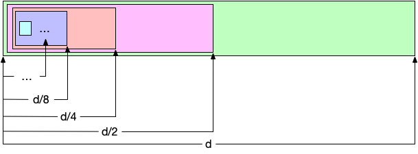
Matryoshka representation learning (MRL) encodes different feature granularities into subsets of a \(d\)-dimensional vector with no additional training or inference cost, all while maintaining similar accuracy with each subset of the features. More specifically, MRL trains \(|{\cal M}| = O(log_2(d))\) subsets of the vector, where \({\cal M}\) contains the feature subsets and each subset is the first \(k \in [1, \dots, d]\) dimensions of the vector. The below figure illustrates the different subsets in \({\cal M}\) that are trained using MRL.
 |
|---|
| Subsets of a feature vector with \(d\) dimensions trained using MRL - Each subset denotes the first \(k\) dimensions of the vector. |
MRL trains each of the the subsets \({\cal M}\) to solve the same task, thus learning features at different scales that can be used to solve the task. In more detail, a \(d\)-dimensional vector \(z\) is acquired by passing a data point \(x \in {\cal X}\) through neural network \(F_{\theta}(\cdot): {\cal X} \rightarrow R^d\) parameterized by \(\theta\). MRL then linearly projects each of the subsets of \(z\) (i.e., \({\cal M}\)) into the task space (classification, regression, etc.) through a set of weights \(\{ W_m | m \in {\cal M} \}\), and trains both \(F\) and the weights over the task’s loss \({\cal L}\). The below equation defines the training objective of MRL:
\[min_{ (W_m | m \in {\cal M}; \theta) } \frac{1}{N} \sum_{i=1}^{N} \sum_{m \in {\cal M}} c_m * {\cal L}(W_m*F_{\theta}(x_i)_{m}, y_i)\]where \((x_i, y_i) \in D\) is point in dataset \(D\), \(F_{\theta}(x_i)_{m}\) denotes feature subset of the representation, and \(c_m\) denotes an importance scaling factor (set to 1 in our experiments).
Model Configuration
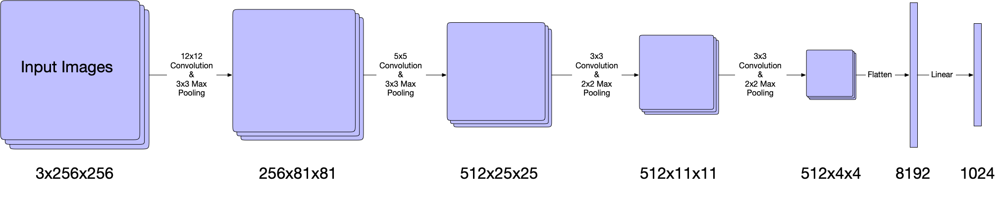
To evaluate and understand how MRL works for a “cats vs. dogs” classification task, I built and trained two models: a baseline model and a MRL model. Both models have the same feature extraction backbone (\(F_{\theta}\) from the previous section) containing four convolutional layers each with max pooling layers and a linear layer. Below is a diagram of the feature extraction backbone:
 |
|---|
| Feature extraction backbone. The backbone uses four convolutional layers with max pooling, whose output is flattened and passed into a linear layer. The output of this linear layer is fed into a classification head for the baseline model or multiple heads for MRL model. |
In more detail, the first convolutional layer has a 12x12 kernel with a 3x3 max pooling layer. This transforms a 3x256x256 image into a 256x81x81 tensor. The second convolutional layer has a 5x5 kernel with a 3x3 max pooling layer, which transforms a 256x81x81 tensor into a 512x25x25 tensor. The third and convolutional layers have a 3x3 kernel with a 2x2 max pooling layer. These transform a 512x25x25 tensor into a 512x4x4. The output of the final convolutional layer is flattened into a vector of dimensions 8192 and passed into a single linear layer of dimensions 1024. This results in the dense representation that will be trained using MRL and used for classification.
The difference between the baseline and MRL models is the classification head. The baseline model uses a single classification head which directly takes the \(d=1024\) dimensional output of the feature extractor to classify cats and dogs. On the other hand, the MRL model uses \(O(log_{2}(d))-2\) = 8 classification heads. I removed the two heads that would intake 2 and 4 features, hence the 8 heads instead of 10 heads. It is possible that we can use 2 and 4 features to classify cats and dogs, but I suspect this will not be the case with more complex datasets that have more animals. I wanted to keep these models as agnostic to the dataset as possible so I can scale the complexity in later work, so I removed those feature subsets.
Experiment Setup
Cats vs. Dogs Dataset
I elected to use the “cats vs. dogs” dataset on HuggingFace.
This dataset is part of the Asirra dataset that was provided by Petfinder.com.
There are two features in the dataset: image and labels.
The image feature consists of images of cats and dogs while the labels denote whether its corresponding image is a cat or dog (0 for cat and 1 for dog).
There are a few characteristics to note about this dataset. The dataset is mostly balanced, with 11,741 cats and 11,669 dogs; however, it is unclear whether there is a balance between cat and dog breeds. Additionally, images in the dataset have varying heights and widths, which means that images will have varying levels of detail. More specifically, there are 3635 unique image dimensions in the dataset, with 412 unique heights and 429 unique widths. The min height and width of an image is 4 while the max height and width is 500.
I viewed images whose dimensions are below 100x100 as noisy; thus I removed them from the dataset prior to training. Even if some are not noise, there may not be enough detail in the image to make classification inferences. I then split the dataset into 90% training and 10% validation, where I kept an balanced split between cats and dogs in each split. Note that I did not create an evaluation dataset. I did not want to use samples from this dataset for evaluation; I will build another dataset for evaluation as next steps.
Model Training
Both models were trained using the same configuration below:
- Epochs: 15
- Batch Size: 8
- Gradient Accumulation Steps: 4
- Learning Rate Scheduler: Exponential Learning Rate Scheduler with decay of 0.85
- Optimizer: AdamW with learning rate of 0.0004 (all other parameters unchanged)
Each image in the training and validation dataset underwent preprocessing prior to being passed into the model. Specifically, the original images were resized into dimensions 3x256x256 and then normalized such that all channel values were in the range (-1, 1). For training, I introduced two data augmentation methods, random horizontal flip and gaussian blur: the training images were randomly flipped horizontally with a probability of 0.5 and passed through a gaussian blur filter with a 3x3 kernel.
Experiment Results
Please note that these results should be taken with a grain of salt; I have not done 5x2 cross validation and any statistical significance tests over these results.
I present a subset of the results from my initial experiment here; the complete set of results can be found on the project’s Weights and Biases page (see Baseline results and MRL results). I trained the models over 15 epochs (39179 training steps) and computed average top-1 accuracy after each training phase to evaluate the performance of the models. First, let’s look at the baseline results. Below is a graph of the validation accuracy over the 15 epochs:
 |
|---|
| Validation accuracy of baseline model. Model performance continued to increase and peaked at epoch 15 with accuracy 0.83 |
The x-axis is denoted by the number of training steps, which is the number of batches times epochs while the y-axis is the average validation accuracy. The baseline validation accuracy hits its max value at epoch 15 with a value of 0.83. We note that the accuracy has not plateaued, implying that increased training time can improve performance.
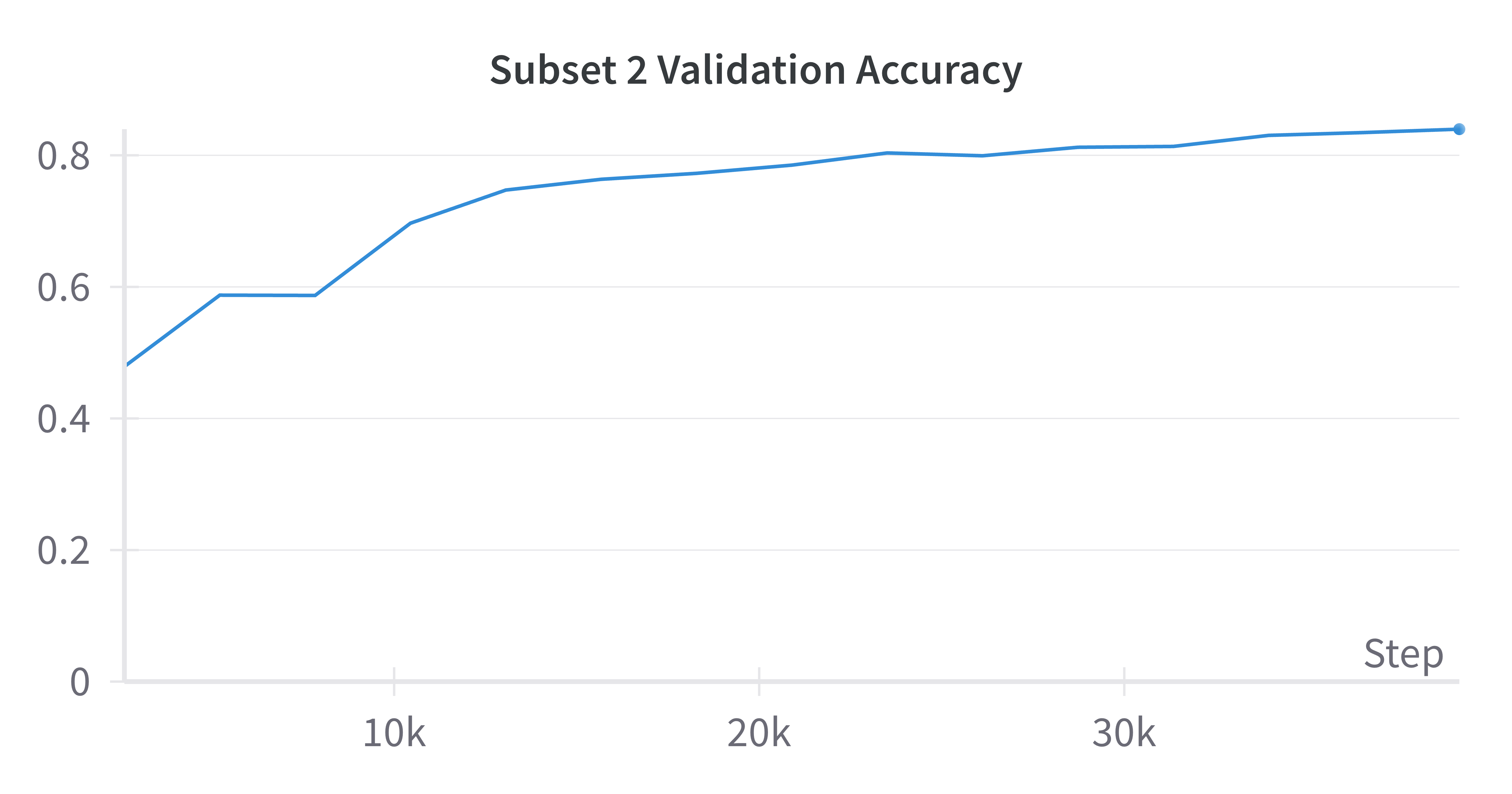
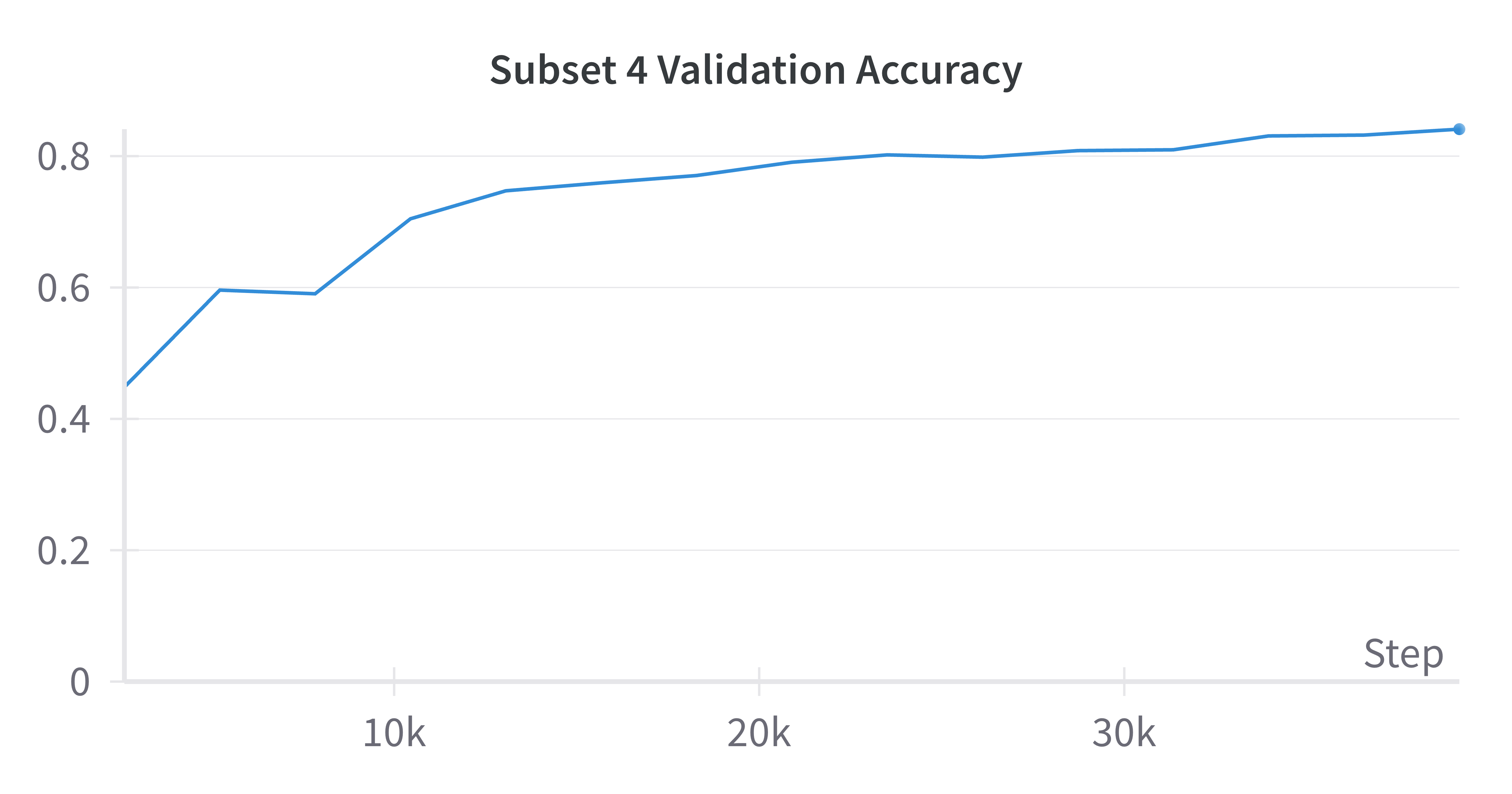
Next, let’s look at the MRL results. Below I provide validation results for half of the feature subsets; the rest can be found on the Weights and Biases project page.
 |
 |
|---|---|
| 8 Features | 16 Features |
 |
 |
| 64 Features | 1024 Features |
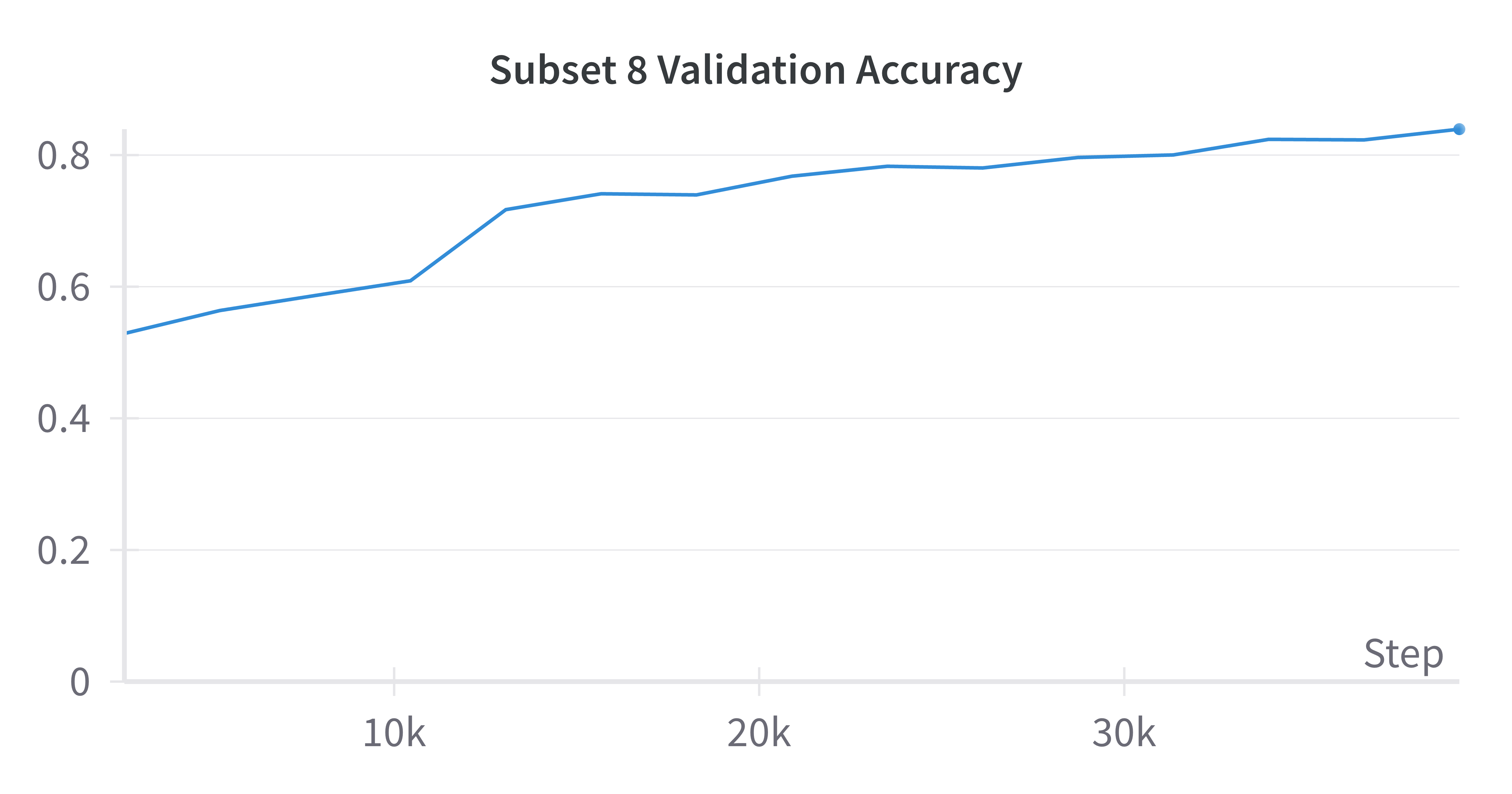
All subsets reached a validation accuracy of 0.84 at epoch 15, which outperforms the baseline model. This is unexpected for the subsets that are smaller than the baseline of 1024 as I expected those to underperform the baseline. I suspect this may be related to each subset learning “generalistic” features that can satisfy subsuming subsets (i.e., subset 1 with 8 features needs to learn features that allow subsets 2 through 8 to perform well). Similar to the baseline results, these graphs indicate that additional training time could improve performance. That said, these results show that even using a small set of features can help with classifying cats and dogs; there is no need to use 1024 features when 8 can suffice.
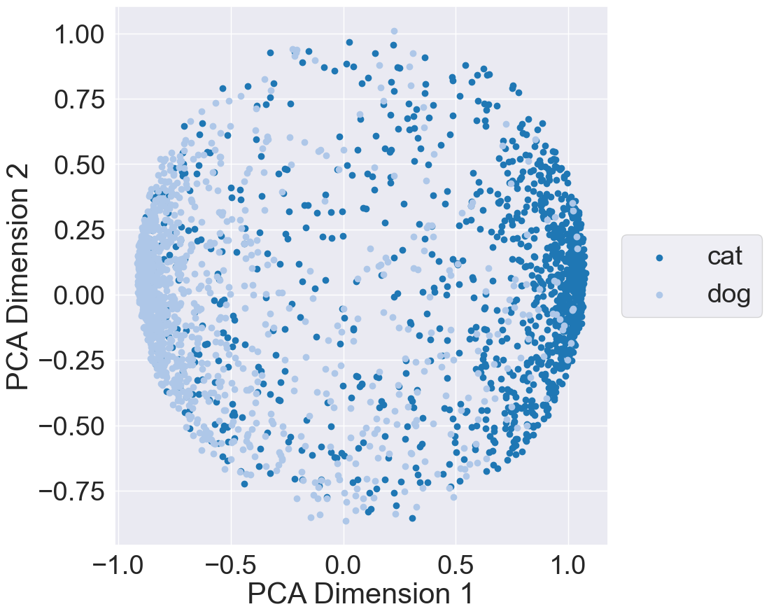
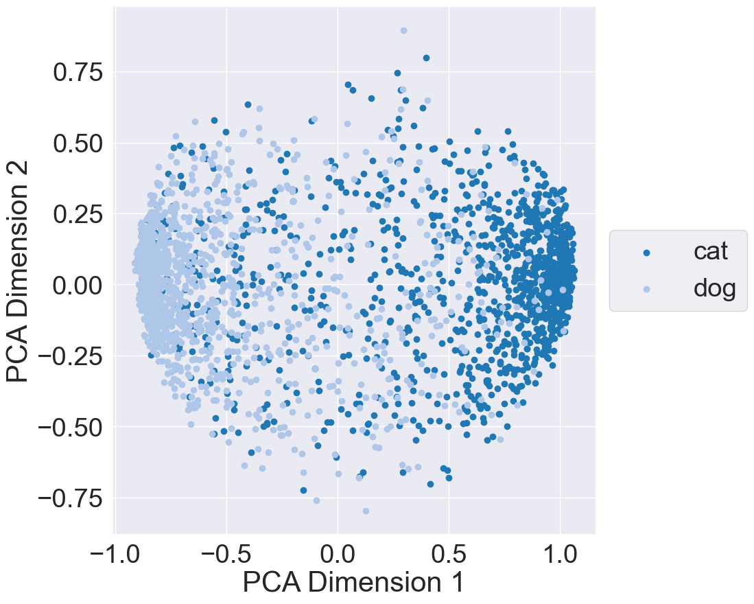
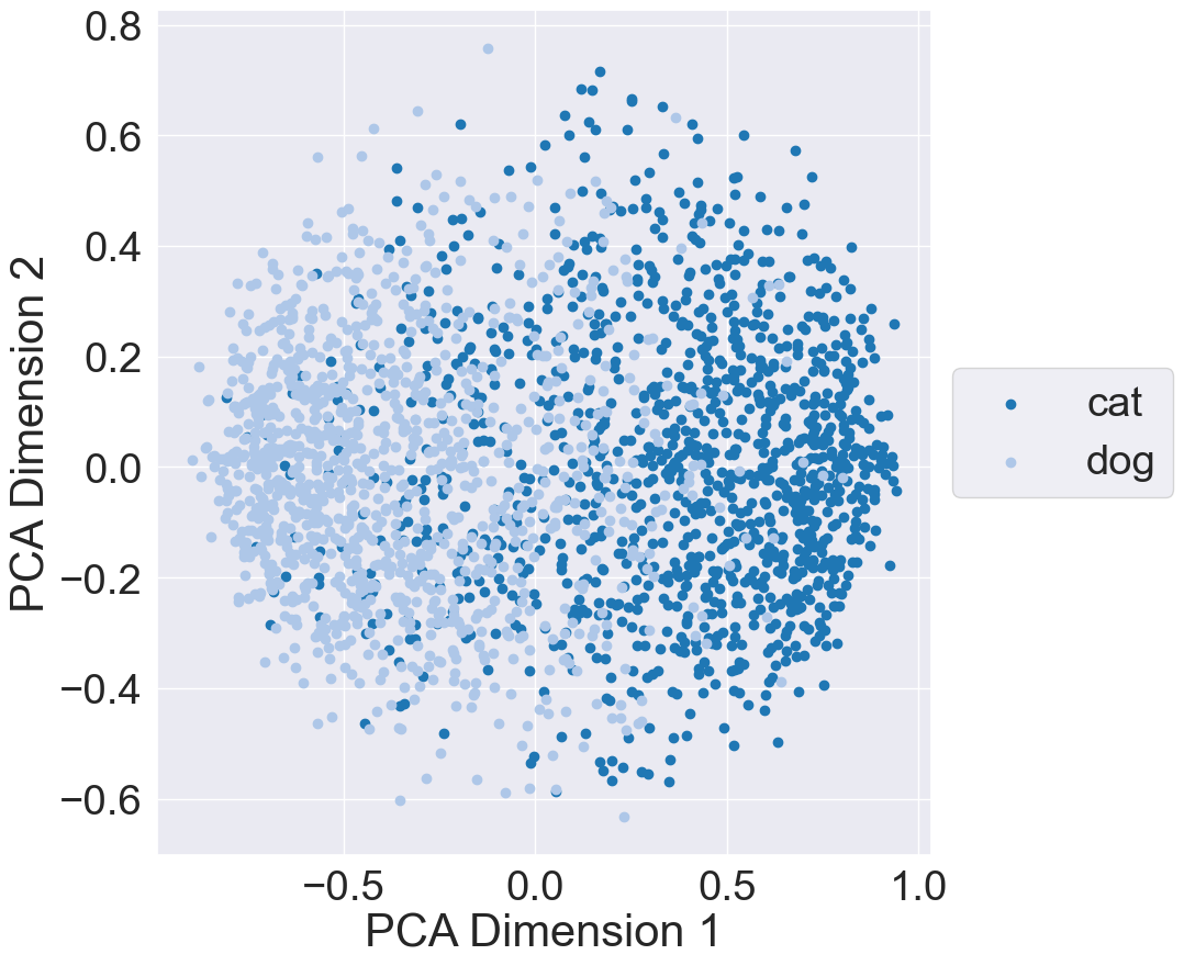
Finally, to better undestand the representation space learned by MRL, I plotted the learned subspace using the validation dataset. More specifically, I passed each validation data point through the MRL model and acquired the outputs of the feature extractor backbone. I then extracted out each subset from the backbone’s outputs and plotted each subset using Principal Component Analysis (PCA): The below plots illustrate the representation space when using 8, 64, 512, and 1024 features from the backbone’s output:
 |
 |
|---|---|
| 8 Features | 64 Features |
 |
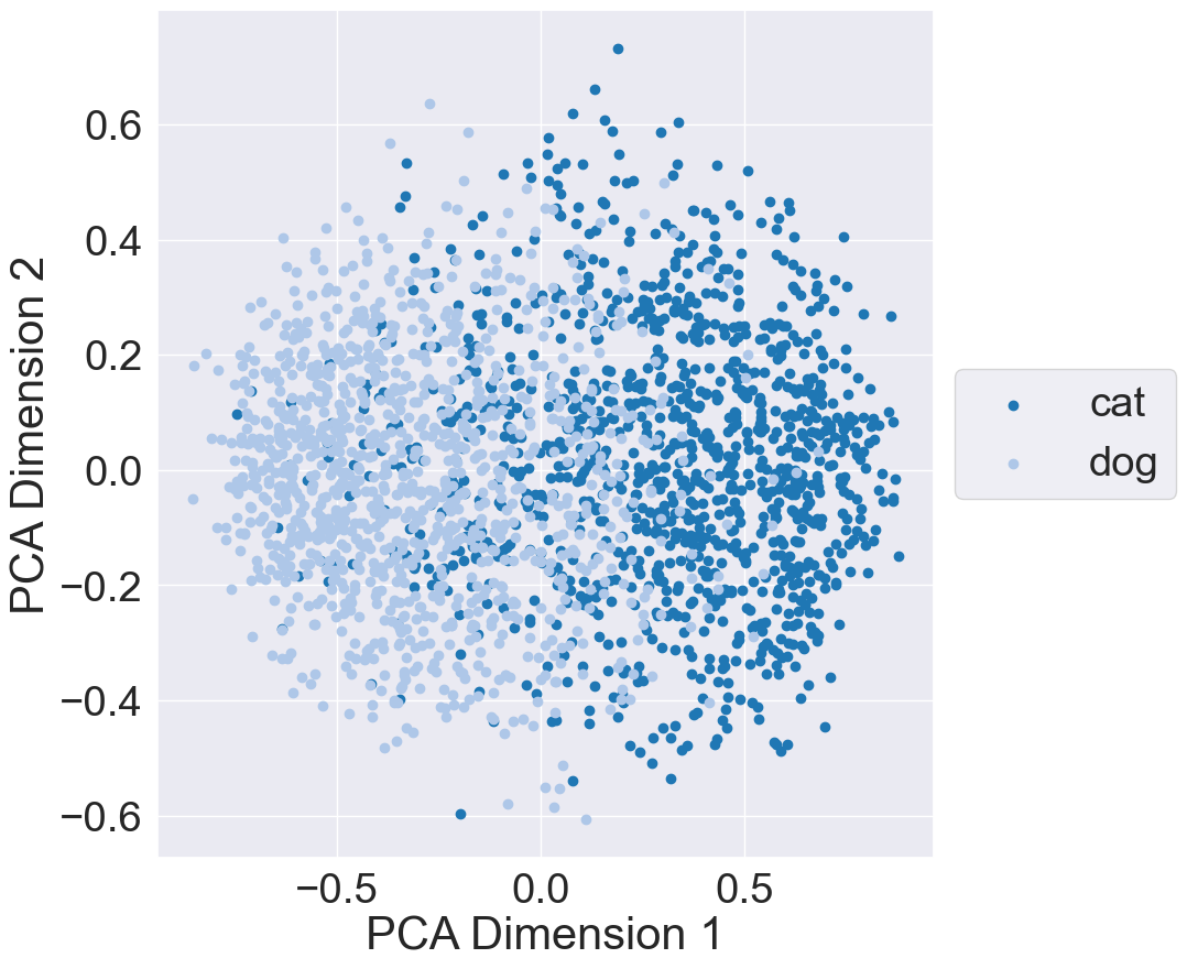 |
| 512 Features | 1024 Features |
These results indicate that 8 features is sufficient to provide a separation between the cat and dog classes. However, we need to be cautious; these 8 features are from MRL training. If we train a model whose feature backbone provides only 8 features, we may get worse separation and performance. Out of curiosity, I trained and evaluated a model whose feature backbone outputs 8 features; results can be found on its Weights and Biases page. The model reaches a maximum validation accuray of 0.83 and has similar class seperation to the 8-feature subset from MRL training.
Conclusion
This blog presents a small study I did on how MRL can be used to train a “cat or dog” classifier. MRL trains a deep convolutional architecture to construct dense representations that can be scaled up or down depending on the compute requirements of downstream applications. My initial results show that we can reduce the number of features needed for classifying cats and dogs by 128x (from 1024 to 8).
There are a few next steps for this project. First, the dataset I used is rather small and contains one type of image (animals); more complex datasets with a large number of animals or different types of images could have different results and I’m interested in seeing how well MRL performs on them. Second, this project focused on image classification and it would be interesting to study other vision tasks such as segmentation or image generation.
Thank you for reading and let me know if you have any questions!